Network Observability

In the previous chapter on Cluster Networking, we explored the implementation of Pod connectivity using CNI plugins and overlay networks like VXLAN. This chapter shifts the focus toward Network Observability, detailing the architecture required to monitor, analyze, and troubleshoot the Kubernetes networking stack. It provides an in-depth look at key network metrics — such as latency, throughput, and packet drops — with an emphasis on the causes and effects of TCP retransmissions. Central to this discussion is a hands-on exploration of kernel-based instrumentation with eBPF, demonstrating how to attach kprobes and tracepoints to extract performance metrics directly from the Linux kernel. Furthermore, it outlines the end-to-end lifecycle of observability data by demonstrating how to correlate cross-layer Pod metrics, store them in time-series databases, and build Grafana dashboards for cluster-level visualization.

Running example

An observability platform can typically monitor several layers (kubernetes_container_networking): Kubernetes, container, Linux, and device layers.

Kubernetes, container, Linux, and devices

Layer	Focus	Technologies
Kubernetes	Pod-to-Pod and service-level traffic management	CNI plugins, network policies
Container	Container-to-container connectivity	Docker bridge network or overlay networks
Linux	Kernel-level network stack and routing	Bridges, veth pairs, iptables, IPVS, conntrack, TC
Device	Hardware-level networking	Switches, routers, NICs

Our running example will bridge the gap between Kubernetes, container, and Linux networking. We will observe the health of inter-Pod (and container) communication by monitoring the number of TCP retransmissions occurring within the Linux network stack, specifically by attaching eBPF programs to kernel functions such as tcp_retransmit_skb.

Architecture

The system to develop consists of four Kubernetes Pods (pod_network_system): pod-a, pod-b, pod-c, and pod-d forming a fully connected network where each Pod communicates with every other Pod through REST API calls. The communication pattern is symmetric, meaning each Pod initiates requests to the three other Pods.

Pod network system.

As every Pod communicates with all others, the system generates \(n(n-1)\) directed communication flows (12 total flows):

• pod-a sends REST calls to pod-b, pod-c, and pod-d.

• pod-b sends REST calls to pod-a, pod-c, and pod-d.

• pod-c sends REST calls to pod-a, pod-b, and pod-d.

• pod-d sends REST calls to pod-a, pod-b, and pod-c.

In complex and large-scale deployments, TCP retransmissions may occur due to packet loss, delay, or network congestion. Because this test deployment is small, we will artificially inject packet loss directly at the network interfaces used by the Pods (such as their virtual Ethernet pairs). This simulates a larger deployment undergoing broader cluster degradation and forces the Linux network stack to trigger TCP retransmissions.

Objectives

The main objectives of this chapter are:

• High-Performance Monitoring with eBPF: Leverage eBPF to monitor kernel events like tcp_retransmit_skb, gaining visibility without the heavy CPU overhead of traditional packet capture tools.

• Contextual Data Correlation: Map low-level kernel IP data to high-level Kubernetes identities, ensuring metrics are tied directly to Pods and Services.

• The Prometheus Stack: Deploy the kube-prometheus stack and configure persistent volumes to ensure long-term data retention.

• ML-Driven Root Cause Analysis: Apply machine learning models to identify correlations between Pod behavior and cascading network retransmissions.

Cluster

We will deploy a dedicated Kubernetes cluster that will serve as our primary infrastructure throughout the remainder of this chapter. Follow the instructions provided in the Cluster Deployment chapter. If you have an existing cluster from a previous session, it is recommended that you tear it down first using the -D flag (cluster_manager.sh -D) to ensure a clean slate.

$ cluster_manager.sh -n 3

The option -n specifies the total number of nodes (one control plane node and n-1 worker nodes).

Once the deployment script completes, verify that all nodes are initialized and reporting a Ready status.

$ kubectl get nodes

NAME            STATUS   ROLES           AGE   VERSION
control-plane   Ready    control-plane   86s   v1.35.3
worker0         Ready    worker          72s   v1.35.3
worker1         Ready    worker          69s   v1.35.3

Linux primitives

Kernel counters

The performance of a Kubernetes cluster can be monitored through Linux kernel counters. common_network_metrics provides an overview of key network metrics. Metrics such as retransmissions, latency, and throughput indicate the health and performance of the network.

Common network metrics

Metric	Description
Packet Drops	Packets discarded by the kernel or NIC (e.g., rx_dropped, qdisc drops)
Packet Loss	Packets lost in transit between nodes, often inferred by TCP via missing ACKs
Throughput	Rate of data transmission across the network, typically in bits per second (e.g., Mbps or Gbps)
Latency	Delay between sending a request and receiving a response (round-trip time, RTT)
Jitter	Variability or fluctuation in packet latency
Retransmissions	Number of packets resent due to errors or losses, e.g., TCP retransmissions
Error Rate	Ratio of packets with errors to total packets transmitted
Connection Failures	Number of failed connection attempts

This chapter focuses on observing TCP retransmissions, which can occur for several reasons. For example, if an acknowledgment (ACK) is not received within the retransmission timeout (RTO) of a segment, TCP assumes packets were lost, possibly due to network congestion, and retransmits them. In response to duplicate ACKs, the sender may trigger a Fast Retransmit, sending missing packets without waiting for the RTO to expire. In some situations, out-of-order packets arrive at the receiver and trigger duplicate ACKs, which may cause the sender to initiate a Fast Retransmit. High retransmission rates typically lead to lower throughput and increased latency, and they consume additional CPU, memory, and bandwidth. Systems involved in communication require additional CPU resources to calculate retransmission timing and handle congestion control.

eBPF

There are several approaches to collecting information on TCP retransmissions: built-in utilities, network monitoring tools, and kernel-based instrumentation.

• Built-in utilities, such as ss -i | grep retrans and netstat -s | grep “segments retransmitted”, provide a human-readable interface to the underlying kernel metrics exposed through virtual files like /proc/net/netstat (specifically under the TcpExt fields) and /proc/net/tcp.

• Network monitoring tools, such as Wireshark and tcpdump, are sophisticated tools for capturing and analyzing packet-level data.

• Kernel-based instrumentation utilizes eBPF to attach custom programs to functions, such as tcp_retransmit_skb, to measure retransmissions at the kernel level. This provides a programmable way to extract data directly from the Linux kernel.

This chapter focuses on kernel-based instrumentation using eBPF (Extended Berkeley Packet Filter). Instead of using traditional tools, which typically poll /proc/net/netstat every few seconds, our eBPF program pushes events to user space in real time, via a BPF perf buffer or ring buffer, allowing us to correlate retransmission spikes with application behavior.

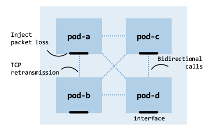
Probe

This section demonstrates how to develop an eBPF-based probe for capturing TCP retransmissions, packaged within a Prometheus exporter to facilitate external metric scraping. The process involves six main steps:

• Attachment points: Identify specific kernel hooks to monitor TCP retransmission events.

• Writing bytecode: Develop the eBPF code required to capture metrics during these events.

• Loading and probing: Inject the bytecode into the kernel to begin data collection via probes.

• Cross-layer correlation: Map captured IP addresses to specific Pods for container-level visibility.

• Exporting metrics: Expose the retransmission data to external applications via an HTTP endpoint.

• Orchestration: Manage the threads for continuous eBPF probing and metadata synchronization.

The following suite of code files forms the core of the system developed. tbl-system-component-breakdown provides a functional breakdown of these components and their roles within the monitoring pipeline.

System component breakdown

Section	Source file	Responsibility
Attachment points	CLI (bpftrace)	Manually investigate candidate attachment points
Writing bytecode	kprobe.c	eBPF program that monitors TCP retransmissions at the kernel level via kprobes
Loading and probing	kprobe.py	Loads the eBPF bytecode and attaches it to the kernel function tcp_retransmit_skb
Cross-layer correlation	kubeinfo.py	Retrieves Pod metadata (names and IPs) from the Kubernetes control plane
Exporting metrics	exporter.py	Formats and pushes TCP retransmission metrics to external monitoring systems
Orchestration	orchestrator.py	Manages the complete application by running concurrent threads that read the eBPF program and correlate raw IP data with Pod identities

architecture_ebpf_probe shows the architecture of the eBPF probe and the responsibilities of each code file.

Architecture of the eBPF probe.

interaction_ebpf_kernel illustrates the interaction between an eBPF program and the kernel. ❶ The user-space program loads an eBPF program and requests attaching it to a specific kernel hook. ❷ The kernel verifies the eBPF program using the eBPF verifier to ensure safety and correctness. ❸ The kernel loads the verified program into kernel space. ❹ The kernel attaches the eBPF program to the specified hook (e.g., tcp_retransmit_skb). ❺ When the hooked kernel function is executed (e.g., during packet retransmission), the eBPF program is triggered. ❻ The eBPF program extracts relevant data from the function arguments or kernel context and computes metrics such as packet or byte counts. ❼ These metrics are stored in BPF maps (kernel-managed shared data structures). Finally, ❽ the user-space program retrieves the metrics by polling or subscribing to updates from the BPF maps.

        sequenceDiagram
    autonumber

    participant user as User-space <br/> program
    participant kernel as Linux kernel
    participant ebpf as eBPF program
    participant kf as Kernel function <br/> e.g., tcp_retransmit_skb
    participant map as BPF maps

    user->>kernel: load eBPF program <br/> + request attachment
    kernel->>kernel: verify program <br/> (eBPF verifier)
    kernel-->>ebpf: load into <br/> kernel space
    kernel->>kf: attach eBPF program <br/> to hook

    kf->>ebpf: trigger on event <br/> (function call)
    ebpf->>ebpf: extract context & compute metrics
    ebpf->>map: store metrics in BPF maps

    loop Polling / retrieval
        user->>map: read metrics
    end
    

Interaction between an eBPF program and the kernel

Following the table, each component and its corresponding source file is described in detail within its own dedicated section.

Attachment points

In eBPF, attachment points are locations in the kernel or user-space applications where programs are attached to observe or modify behavior. attachment_points shows various attachment points in the Linux kernel.

Attachment points for eBPF programs

Location	Description
Tracepoints	Static points managed by kernel developers that are generally stable across kernel versions.
Kprobes / kretprobes	Kernel probes can be affected by kernel changes. Kretprobes are attached to the return of functions (see /proc/kallsyms).
Uprobes / Uretprobes	User-space probes are similar to kprobes, but they are attached to user-space functions. Uretprobes are attached to the return of functions.

To operate these attachment points, eBPF provides a framework and interfaces that exist in the Linux kernel. ebpf_framework lists the most relevant files. For example, header files such as bpf.h and filter.h provide definitions and structures required for eBPF program execution.

eBPF interfaces in the Linux kernel

File	Purpose
include/linux/bpf.h	Definitions of eBPF program types and data structures for managing eBPF maps and programs.
include/uapi/linux/bpf.h	User-space API for interacting with eBPF and map types visible to user-space.
include/linux/filter.h	Macros and structures used to interpret and execute BPF programs.
include/uapi/linux/filter.h	Definitions for the classic BPF (cBPF) and socket filtering macros.
kernel/bpf/syscall.c	System calls related to eBPF, such as loading and unloading programs and managing maps.
kernel/bpf/core.c	BPF virtual machine (interpreter) that executes eBPF bytecode.
kernel/bpf/verifier.c	BPF verifier to check for program correctness.
net/core/filter.c	Functions for networking, e.g., TC (Traffic Control) and XDP (eXpress Data Path).
kernel/trace/bpf_trace.c	Functions for tracing, e.g., kprobes and tracepoints.
net/sched/act_bpf.c	Manages BPF actions in the TC.
net/sched/cls_bpf.c	Manages BPF filters in the TC.

The bpftrace tool can be used to find kprobes and tracepoints of interest to measure TCP retransmissions. This tool allows one to write small scripts to trace system behavior and performance (e.g., monitoring disk I/O latency and tracing syscall activity) in a user-friendly language inspired by C and AWK. The following example illustrates how to use the tool to list all available kprobes that match the pattern tcp*retransmit* in their names:

$ sudo bpftrace -l "kprobe:tcp*retransmit*"

kprobe:tcp_non_congestion_loss_retransmit
kprobe:tcp_retransmit_skb
kprobe:tcp_retransmit_timer
kprobe:tcp_simple_retransmit
kprobe:tcp_xmit_retransmit_queue

A similar command can be executed to list the tracepoints:

$ sudo bpftrace -l "tracepoint:tcp*"

tracepoint:tcp:tcp_bad_csum
tracepoint:tcp:tcp_cong_state_set
tracepoint:tcp:tcp_destroy_sock
tracepoint:tcp:tcp_probe
tracepoint:tcp:tcp_rcv_space_adjust
tracepoint:tcp:tcp_receive_reset
tracepoint:tcp:tcp_retransmit_skb
tracepoint:tcp:tcp_retransmit_synack
tracepoint:tcp:tcp_send_reset

Unlike kprobes, since tracepoints are predefined hooks within the kernel source code, they have predefined data structures which can be listed using the bpftrace tool. For example, to show the arguments and data format provided by the tracepoint tracepoint:tcp:tcp_retransmit_skb:

$ sudo bpftrace -lv "tracepoint:tcp:tcp_retransmit_skb"

tracepoint:tcp:tcp_retransmit_skb
    const void * skbaddr
    const void * skaddr
    int state
    __u16 sport
    __u16 dport
    __u16 family
    __u8 saddr[4]
    __u8 daddr[4]
    __u8 saddr_v6[16]
    __u8 daddr_v6[16]

From all the attachment points previously identified, two kprobes seem to be of interest to measure TCP retransmissions: tcp_retransmit_skb and tcp_retransmit_timer. The main files governing the TCP state machine and retransmissions are located within the core net/ipv4/ directory (which handles basic TCP logic for both IPv4 and IPv6 dual-stack operations):

• tcp_retransmit_skb: This function is called when the kernel retransmits a TCP segment. It is located in the file net/ipv4/tcp_output.c.

• tcp_retransmit_timer: This function schedules retransmissions when ACKs are not received within a certain time. It is located in the file net/ipv4/tcp_timer.c.

We can use bpftrace to trace the tcp_retransmit_skb kernel function via a kprobe and print a message whenever this function is triggered.

sudo bpftrace -e '
  kprobe:tcp_retransmit_skb {
    printf("Retransmission: %s\n", comm);
  }
'

Attaching 1 probe...
Retransmission: swapper/2
Retransmission: swapper/2
...

We can do the same to trace events related to TCP retransmissions via a tracepoint and print the process ID (PID) of the process initiating the retransmission.

sudo bpftrace -e '
  tracepoint:tcp:tcp_retransmit_skb {
    printf("Retransmission from PID %d\n", pid);
  }
'

Attaching 1 probe...
Retransmission from PID 0
Retransmission from PID 0
...

Note

The retransmissions report swapper/2 or PID 0. This indicates that the retransmission was triggered asynchronously by a software interrupt (SoftIRQ) or timer expiration while the CPU was executing its idle task (PID 0), rather than directly by an active user-space application thread.

From our investigation, both kprobes and tracepoints can capture TCP retransmissions. While the tcp_retransmit_skb tracepoint is stable and preferred for production, we will use kprobes to demonstrate how to access raw kernel function signatures and internal socket structures (struct sock *sk) that are not fully exposed through standard tracepoint definitions.

Writing bytecode

After identifying the instrumentation point within the kernel, the next step is to develop the eBPF source code responsible for capturing the telemetry. The eBPF program kprobe.c, shown below and written in C, tracks the total retransmissions for each unique TCP flow, identified by the 4-tuple (source/destination IP, ports).

struct flow_key_t {
    __be32 src_ip;
    __be32 dst_ip;
    __be16 src_port;
    __be16 dst_port;
};

BPF_HASH(rtx_count, struct flow_key_t, u64);

int count_tcp_retransmit(struct pt_regs *ctx) {
    struct sock *sk;
    struct flow_key_t flow_key = {};
    u64 *count, zero = 0;

    sk = (struct sock *)PT_REGS_PARM1(ctx);
    if (!sk)
        return 0;

    // Extract source and destination IPs and ports
    bpf_probe_read_kernel(&flow_key.src_ip, sizeof(flow_key.src_ip), &sk->sk_rcv_saddr);
    bpf_probe_read_kernel(&flow_key.dst_ip, sizeof(flow_key.dst_ip), &sk->sk_daddr);
    bpf_probe_read_kernel(&flow_key.src_port, sizeof(flow_key.src_port), &sk->sk_num);
    bpf_probe_read_kernel(&flow_key.dst_port, sizeof(flow_key.dst_port), &sk->sk_dport);

    // Swap byte order of destination port
    flow_key.dst_port = ntohs(flow_key.dst_port);

    // Update retransmission counter for this flow
    count = rtx_count.lookup_or_try_init(&flow_key, &zero);
    if (count) {
        (*count)++;
    }

    return 0;
}

The function count_tcp_retransmit is called when a TCP retransmission occurs. The flow information is extracted from the socket structure (typically struct sock * or struct tcp_sock *), a pointer to a kernel-level structure that holds information about a network socket. The function stores counts in an eBPF map (rtx_count). The key is defined by the flow_key_t structure, which includes the source IP, destination IP, source port, and destination port. The value is the retransmission count, stored as an unsigned 64-bit integer (u64).

Loading and probing

The Python file kprobe.py loads the eBPF source code from the previous section and attaches it to the kernel function tcp_retransmit_skb to trace retransmissions. The script has three main parts:

• Reading the eBPF C program from a file.

• Loading the program into the BPF context.

• Polling the perf buffer to retrieve data.

def probe(b, func_record, timeout=1000):
    """Pool perf buffer for data."""
    rtx_count = b["rtx_count"]
    logger.info("Probe called. Number of records: %d", len(rtx_count.items()))
    for flow, count in rtx_count.items():
        func_record(int_to_ip(flow.src_ip),
                    int_to_ip(flow.dst_ip),
                    flow.src_port,
                    flow.dst_port,
                    count.value)

    rtx_count.clear()
    b.perf_buffer_poll(timeout=timeout)

The two main functions are load_bpf_program and probe:

• load_bpf_program(): This function loads the eBPF program and attaches it to a kernel probe. This creates a BPF object to interact with the kernel. The kprobe is instrumented at the entry point of the tcp_retransmit_skb kernel function. The function returns the BPF object (referred to as b in the code), which represents the loaded eBPF program.

• probe(…): This function polls the perf buffer for data and processes the TCP retransmission counts per flow. func_record(…) is a callback function that processes the flow data. The script uses the rtx_count BPF map to store persistent counters, while b.perf_buffer_poll(…) is used to asynchronously stream event-level data to user space.

To receive the data collected by the probe, the manager passes a callback function called func_record. The function is then called every time the perf buffer has data.

Cross-layer correlation

The Python script kubeinfo.py bridges the gap between the kernel and the cluster by mapping network retransmission data collected by the eBPF bytecode to specific Kubernetes Pod names — a correlation the bytecode cannot perform on its own using only raw IP addresses.

The script retrieves information about Pods using the Kubernetes Python client to call the Kubernetes API, obtaining Pod names and their IPs.

def update_pod_info(namespace="default"):
    """Queries Kubernetes API to get pod names and IPs."""
    global pod_info_dict

    if not KUBERNETES_CONGIGURED:
        return
    
    try:
        pods = v1.list_namespaced_pod(namespace)
        pod_info_dict.clear()
        for pod in pods.items:
            pod_name = pod.metadata.name
            pod_ip = pod.status.pod_ip
            pod_info_dict[pod_ip] = pod_name
        logger.info(f"Updated information of {len(pod_info_dict)} pods")
        for ip, name in pod_info_dict.items():
            logger.info(f"Pod Name: {name} ({ip})")
    except Exception as e:
        logger.error(f"Error querying Kubernetes: {e}")

def get_pod_name_by_ip(pod_name):
    """Retrieves the IP of a pod from the using the pod's name."""
    return pod_info_dict.get(pod_name, None)

The program uses the Kubernetes configuration file (e.g., /home/ubuntu/.kube/config) to initialize the client. The two main functions are update_pod_info and get_pod_name_by_ip:

• update_pod_info(): This function queries the Kubernetes API to retrieve a list of pods. The list is stored in the dictionary pod_info_dict, which maps Pod IPs to Pod names. The dictionary is updated periodically by a background management loop that calls update_pod_info().

• get_pod_name_by_ip(pod_ip): This function retrieves a Pod’s name given its IP by accessing the pod_info_dict dictionary.

In specific scenarios, a Pod can be configured to use the host’s network namespace. The Pod IP address will correspond to the underlying node’s IP due to the network setup (hostNetwork is true in the Pod’s spec). In such scenarios, the Pod’s IP will be the same as the node’s IP.

Exporting metrics

The Python script exporter.py exports the TCP retransmission count metric using the Prometheus format.

def record_retransmissions(src_ip, dst_ip, src_port, dst_port, count):
    """Record retransmission data to Prometheus."""
    src_pod_name = get_pod_name_by_ip(src_ip) or src_ip
    dst_pod_name = get_pod_name_by_ip(dst_ip) or dst_ip

    rtx_counter.labels(src_ip=src_ip, dst_ip=dst_ip,
                       src_port=src_port, dst_port=dst_port).inc(count)
    logger.info(f"Recorded retransmission for "
                f"{src_pod_name} ({src_ip}:{src_port}) -> "
                f"{dst_pod_name} ({dst_ip}:{dst_port}), Count: {count}")

def start_prometheus_server(port=9191):
    """Start the Prometheus metrics HTTP server."""
    start_http_server(port, addr='0.0.0.0')
    msg = f"Prometheus metrics server started on port: {port}"
    print(msg)
    logger.info(msg)


start_prometheus_server()

The script uses the prometheus_client library to expose the metric named tcp_retransmissions of type Counter.

• record_retransmissions(…): This function is the callback function passed to the probe by the manager. It sends retransmission data to the Prometheus counter by incrementing it. Since the probe is unable to retrieve the names of the Pods involved in a retransmission, the function also calls get_pod_name_by_ip(…) to resolve IPs into Pod names, which are then added as labels. The metric uses the labels for source and destination IPs and service names (if available).

• start_prometheus_server(…): This function starts an HTTP server on port 9191 to expose the metric to be scraped by a Prometheus server. The port for a Prometheus exporter is typically chosen from the range 9100-9999.

While Prometheus is the industry standard for cloud-native monitoring, several alternatives exist depending on whether you need better scalability or unified logs and traces. For example, VictoriaMetrics, Mimir, or InfluxDB.

Orchestration

The orchestrator.py script is the central orchestrator for the monitoring system. It uses a multi-threaded architecture to synchronize low-level kernel events with high-level container orchestration data. By running concurrent threads, the program simultaneously manages the lifecycle of the eBPF probes and the retrieval of Kubernetes metadata. It relies on eBPF to track retransmissions and periodically updates Pod information to correlate the retransmission data with Pods.

def pod_info_thread():
    logger.info("Starting pod_info_thread... ")
    while True:
        update_pod_info()
        time.sleep(60)


def probe_thread():
    global bpf_program
    logger.info("Starting probe_thread... ")    
    while True:
        probe(bpf_program, record_retransmissions)
        time.sleep(1)


def monitor_threads(threads):
    """Monitors the threads tocheck they are running."""
    print("Manager started: counting TCP retransmissions per flow..."
          "Press Ctrl+C to exit.")
    try:
        while True:
            time.sleep(2)
            for thread in threads:
                if not thread.is_alive():
                    print(f"Thread {thread.name} failed or not running.")
                    sys.exit(1) 
    except KeyboardInterrupt:
        print("Stopping threads...")
        for thread in threads:
            print(f"Stopping thread: {thread.name}")
        sys.exit(0)


def main():
    global bpf_program
    
    logger.info("Starting manager... ")

    try:
        # Load BPF inside the try block so we can log the failure
        bpf_program = load_bpf_program()
    except Exception as e:
        logger.error(f"Failed to load BPF program: {e}")
        sys.exit(1)

    threads = []
    for i, name in [(pod_info_thread, "pod_info"), (probe_thread, "probe")]:
        thread = threading.Thread(target=i, name=name, daemon=True)
        threads.append(thread)
        thread.start()

    monitor_threads(threads)


if __name__ == "__main__":
    main()

The script has three main functions:

• load_bpf_program(): This function loads the eBPF program previously described to monitor TCP retransmissions.

• pod_info_thread(): This function regularly calls the update_pod_info() function to update available Pod names and their associated IP addresses.

• probe_thread(): This function calls the probe() function, which retrieves retransmission data from the kernel via a perf buffer and sends it to the exporter.

The program and the threads can be interrupted by pressing Ctrl+C; the KeyboardInterrupt exception is caught, and the threads are stopped.

In a production environment, because the eBPF probe must hook into the host kernel, it is typically deployed as a DaemonSet to ensure it runs on every node in the cluster. To facilitate monitoring, the probe’s exporter can be wrapped in a Kubernetes Service (e.g., probe.monitoring.svc.cluster.local). The Prometheus config can use the Service DNS, which prevents you from having to manually update Prometheus every time a node’s IP changes. Since the probe interacts with the host’s network stack, the Pod running the orchestrator will use hostNetwork: true in its specification.

Validation

To validate the eBPF orchestrator’s monitoring capabilities, execute the following procedure to simulate network degradation and verify metrics collection.

1. Deploy Pod: Deploy the netshoot container to a specific node (worker0). This Pod is used to generate network traffic.

kubectl run netshoot --privileged --image=nicolaka/netshoot --rm -it \
    --overrides='
  {
    "apiVersion": "v1",
    "spec": {
      "nodeName": "worker0"
    }
  }' \
  -- /bin/bash

Run a curl request to an external endpoint every 2 seconds inside the netshoot container. This ensures there is an active flow for the probe to monitor.

$ watch -n 2 "curl -s http://www.google.com"

2. Initialize Orchestrator: On worker0, launch the probe orchestrator. This script attaches to the kernel to track TCP retransmissions across all network flows and exposes them via a Prometheus-compatible endpoint.

$ python3 -m venv .venv --system-site-packages
$ .venv/bin/pip install -r requirements.txt
$ sudo .venv/bin/python3 orchestrator.py

Prometheus metrics server started on port: 9191
Manager started: counting TCP retransmissions per flow...Press Ctrl+C to exit.

3. Inject Packet Loss: Use the Traffic Control (tc) utility and the Network Emulator (netem) discipline to simulate a degraded network environment by dropping 20% of outgoing packets on the primary interface. On the worker0 node, apply the packet loss to the primary interface (e.g., ens3).

$ sudo tc qdisc add dev ens3 root netem loss 20%

Note: You can also run tc inside the netshoot container or targeted at the Pod’s specific virtual interface (veth pair) on the host.

4. Verify Retransmission Metrics: Retrieve the IP address assigned to the netshoot Pod.

$ POD_IP=$(kubectl get pod netshoot -o jsonpath='{.status.podIP}')

Query the Prometheus metrics endpoint and filter for the Pod’s IP. This confirms that the orchestrator is successfully detecting the TCP retransmissions caused by the injected packet loss.

$ curl -s localhost:9191 | grep $POD_IP

tcp_retransmissions_total{dst_ip="10.244.1.45", ...} 1.0
tcp_retransmissions_created{dst_ip="10.244.1.45", ...} 1.77...+09

Note: In OpenMetrics/Prometheus standards, a _created suffix usually refers to a timestamp (Unix epoch) of when the counter was initialized.

5. Cleanup: Finally, remove the packet loss emulation to restore network reliability.

$ sudo tc qdisc del dev ens3 root netem

Telemetry ingestion

Several systems can be used to store time-series observability data. Notable alternatives include Prometheus, InfluxDB, Graphite, OpenTSDB, VictoriaMetrics, and TimescaleDB. The selection is based on integration capabilities, scalability, performance, and storage capacity requirements. We will illustrate how to deploy Prometheus in Kubernetes and retrieve network metrics from the eBPF probe previously developed. telemetry_ingestion shows the telemetry ingestion architecture using Prometheus.

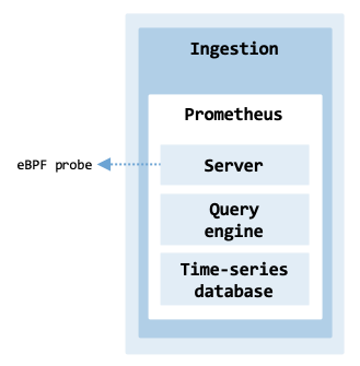
Telemetry ingestion architecture.

Its main components include:

• Server: Responsible for scraping metrics from configured targets, storing them, and providing a query interface. It pulls metrics from exporters or instrumentation libraries that are deployed on nodes, services, and applications.

• Query engine: The query engine uses the PromQL language to retrieve and aggregate time-series data from Prometheus.

• Time-Series Database: Stores the scraped metrics for efficient querying and retrieval.

The script prometheus_manager.sh installs Prometheus. It contains most of the commands described in the following sections. It assumes that the probe is running on the worker0 node on port 9191.

$ prometheus_manager.sh install
$ prometheus_manager.sh uninstall

Installation

There are two options to install Prometheus in a Kubernetes cluster: using a Helm chart or a Prometheus Operator. This section describes how to use a Helm chart to set up the “classic” stack, which deploys Prometheus and Alertmanager.

When deploying Prometheus, use a separate namespace named monitoring instead of the default namespace.

$ kubectl create namespace monitoring
$ kubectl config set-context --current --namespace=monitoring

Create a PersistentVolume definition file (prometheus-pv.yaml) to enable Prometheus to store local data. The resource allocates 10 Gi of capacity on the local filesystem at /mnt/data/prometheus. Only one node can write at a time (ReadWriteOnce) and the data is kept after the PV is released from its PV claim (Retain). The storageClassName is set to an empty string since the definition uses the hostPath — the path on the host machine.

apiVersion: v1
kind: PersistentVolume
metadata:
  name: prometheus-pv
spec:
  capacity:
    storage: 10Gi
  volumeMode: Filesystem
  accessModes:
    - ReadWriteOnce
  persistentVolumeReclaimPolicy: Retain
  storageClassName: ""
  hostPath:
    path: /mnt/data/prometheus
    type: DirectoryOrCreate

Since a PersistentVolume can only be bound to one PersistentVolumeClaim at a time, and Prometheus and Alertmanager are distinct services with different data storage needs, a second volume needs to be created for Alertmanager (alertmanager-pv.yaml).

$ kubectl apply -f prometheus-pv.yaml
$ kubectl apply -f alertmanager-pv.yaml

While the directories specified under the hostPath are created automatically, they are owned by the root user of the host node. Thus, permissions need to be set on worker nodes worker0 and worker1:

for worker in worker0 worker1; do
  for dir in /mnt/data/prometheus /mnt/data/alertmanager; do
    multipass exec "$worker" -- sudo mkdir -p "$dir"
    multipass exec "$worker" -- sudo chown -R 65534:65534 "$dir"
    multipass exec "$worker" -- sudo chmod -R 775 "$dir"
  done
done

The specific UID/GID 65534 is a standard convention to represent the “nobody” user and the “nogroup” group.

Note: If the container user ID doesn’t match the host directory owner, Prometheus will fail with a “Permission Denied” error when attempting to write its TSDB lock file.

Create a configuration file (prometheus-values.yaml) to configure the Prometheus deployment on Kubernetes. The configuration disables the pushgateway and uses the persistent volume prometheus-pv previously created. It uses a NodePort instead of a ClusterIP. The Prometheus server is accessible via any node’s IP on port 30090, which maps to the internal service port 9090. The Alertmanager server is exposed via NodePort 30093 on port 9093. The deployment uses a StatefulSet, ensuring a stable identity and storage for Prometheus. One scrape job is defined for scraping metrics from Prometheus itself.

alertmanager:
  enabled: true
  service:
    port: 9093
    type: NodePort
    nodePort: 30093
  persistence:
    enabled: true
    storageClass: ""
    accessModes:
      - ReadWriteOnce
    size: 1Gi
prometheus-pushgateway:
  enabled: false
server:
  service:
    servicePort: 9090
    type: NodePort
    nodePort: 30090
  persistentVolume:
    enabled: true
    storageClass: ""
    accessModes:
      - ReadWriteOnce
    size: 8Gi 
  statefulSet:
    enabled: true

extraScrapeConfigs: |
  - job_name: 'ebpf-probe'
    static_configs:
      - targets: ['10.30.45.182:9191']

Add the Prometheus Community repository to the local Helm installation (make sure Helm is installed).

$ helm repo add prometheus-community https://prometheus-community.github.io/helm-charts
$ helm repo update

Search for charts that match the keyword “prometheus”:

$ helm search repo prometheus-community/prometheus

NAME                                                 CHART VERSION    ...
prometheus-community/prometheus                      25.23.0
prometheus-community/prometheus-adapter              4.10.0
prometheus-community/prometheus-blackbox-exporter    8.17.0
prometheus-community/prometheus-cloudwatch-expo...   0.25.3
...

Install Prometheus using the customized configuration:

helm install prometheus prometheus-community/prometheus \
    -f prometheus-values.yaml

Check the status of all the objects created in the namespace:

$ kubectl get pods -o wide

NAME                                            READY ...
prometheus-alertmanager-0                       1/1
prometheus-kube-state-metrics-86969d697f-m7rwn  1/1
prometheus-prometheus-node-exporter-4rmcd       1/1
prometheus-prometheus-node-exporter-fp2q7       1/1
prometheus-server-0                             2/2
...

While the Pods exist within the overlay network, the node-exporter Pods are running with hostNetwork: true. The exporter needs to measure the health of the actual physical (or virtual) machine, not just the container. To see the “real” hardware metrics (like disk I/O, network traffic, and CPU load), it bypasses the Kubernetes virtual network and binds directly to the node’s IP address.

Use curl on the control-plane node’s IP address to fetch Node Exporter metrics:

$ curl 192.168.64.27:9100/metrics

Web access

The Prometheus and Alertmanager services are exposed within the cluster on service ports 9090 and 9093, respectively. To access the servers from a cluster node, the node ports are 30090 and 30093.

The Prometheus server can be accessed via port 9090 on the following DNS name from within the cluster:

prometheus-server.monitoring.svc.cluster.local

From the main host running multipass, the web page can be accessed via curl using the node port 30090:

export NODE_PORT=$(
  kubectl get --namespace monitoring \
    -o jsonpath="{.spec.ports[0].nodePort}" \
    services prometheus-server
)
export NODE_IP=$(
  multipass info control-plane | awk '/IPv4/ {print $2}'
)
curl -X OPTIONS -i "http://$NODE_IP:$NODE_PORT"

HTTP/1.1 200 OK
Allow: GET, OPTIONS
Date: Sun, 29 Mar 2026 13:44:52 GMT
Content-Length: 0

The Alertmanager can be accessed via port 9093 on the following DNS name from within the cluster:

prometheus-alertmanager.monitoring.svc.cluster.local

From the main host running multipass, the webpage can be accessed via curl using the node port 30093:

export NODE_PORT=$(kubectl get --namespace monitoring \
      -o jsonpath="{.spec.ports[0].nodePort}" services prometheus-alertmanager)
export NODE_IP=$(multipass info control-plane | awk '/IPv4/ {print $2}')
echo "curl http://$NODE_IP:$NODE_PORT"

Since cluster nodes usually do not have a UI, it is useful to forward the ports from the cluster nodes to the physical host. Specifically, an SSH tunnel can be established by forwarding the cluster node port 30090 to the local port 9090. The same applies to the Alertmanager server, which runs on port 9093.

On the host running multipass, establish two tunnels to the control-plane node.

PROMETHEUS_PORT=9090
ALERTMANAGER_PORT=9093
NODE_IP=$(multipass info control-plane | awk '/IPv4/ {print $2}')
ssh -fN -g -L $PROMETHEUS_PORT:127.0.0.1:30090 \
           -L $ALERTMANAGER_PORT:127.0.0.1:30093 ubuntu@$NODE_IP

The -g flag allows remote hosts (other computers on your local network) to connect to the forwarded ports on your host. The command assumes the user has SSH keys configured for ubuntu@$NODE_IP. Using a browser, access http://localhost:9090/ and http://localhost:9093/.

Once the tunnels are no longer needed, you can remove them using the command:

$ kill $(lsof -t -i:$PROMETHEUS_PORT)

Since we established both port forwards within a single SSH session, it is sufficient to kill the single process.

Scraping metrics

Unfortunately, it is not possible to create or modify scraping endpoints directly from the Prometheus UI. Prometheus configuration is managed via Kubernetes ConfigMaps, which in this deployment are controlled by Helm.

First, obtain the IP address of worker0 where the probe is running:

$ multipass info worker0 | awk '/IPv4/ {print $2}'

10.30.45.224

Update the file prometheus-values.yaml to include the scrape configuration for the eBPF probe under the extraScrapeConfigs key:

extraScrapeConfigs: |
  - job_name: 'ebpf-probe'
    static_configs:
      - targets: ['10.30.45.224:9191']

Apply the changes using Helm:

$ helm upgrade prometheus prometheus-community/prometheus -f prometheus-values.yaml

Finally, verify that the configuration has been successfully injected into the Prometheus server:

$ kubectl exec prometheus-server-0 -c prometheus-server -- \
      cat /etc/config/prometheus.yml | grep 9191

- targets: ['10.30.45.224:9191']

Note: Always use helm upgrade to modify configurations. Manual edits to the ConfigMap via kubectl edit will be overwritten the next time Helm performs a deployment or rollback.

Queries

Prometheus’s query language is called PromQL (Prometheus Query Language). It is used to retrieve and manipulate data stored in Prometheus and offers functionality for filtering, aggregating, and visualizing time-series data.

The simplest query consists of writing tcp_retransmissions_total in the Prometheus UI. The query retrieves all collected data points from the eBPF probe developed earlier. While simple, analyzing the data in more detail can be complex.

tcp_retransmissions_total

A more meaningful query calculates the total number of TCP retransmissions that occurred between two specific IP addresses in a Kubernetes cluster. In the probe we developed, the tcp_retransmissions_total counter is incremented each time a TCP packet is retransmitted due to network issues (e.g., dropped packets).

sum(tcp_retransmissions_total{src_ip="10.244.92.143", dst_ip="10.244.92.144"})

The labels src_ip and dst_ip filter for retransmissions where the source IP is 10.244.92.143 and the destination IP is 10.244.92.144, respectively. Together, these labels ensure the query focuses only on retransmissions between these two specific IP addresses. The function sum aggregates (sums) the values of all time series matching the metric and labels. If the query returns a value of 50, this indicates there have been 50 TCP retransmissions from 10.244.92.143 to 10.244.92.144 since the start of metric collection.

If a more global analysis of the communication within the cluster is needed, the total number of TCP retransmissions for every source-destination IP pair needs to be calculated. It is particularly useful for identifying specific source-destination pairs with a high number of retransmissions, which indicate issues with communication reliability between different nodes of the cluster, possibly separated by different physical networks.

sum(tcp_retransmissions_total) by (src_ip, dst_ip)

The query aggregates the total retransmissions per unique combination of src_ip and dst_ip. The query creates separate groups for each unique combination of source IP src_ip and destination IP dst_ip, producing a result for each pair to show the total retransmissions per flow. It then sums the values of the metric within each group. The result is shown in prometheus_sum.

Number of TCP retransmissions grouped by source and destination IP.

To calculate the per-second average rate of TCP retransmissions per unique source and destination IP pair, we apply a combination of the functions sum() and rate():

sum(rate(tcp_retransmissions_total[5m])) by (src_ip, dst_ip)

The example computes the average per-second increase of retransmissions over a 5-minute period. If tcp_retransmissions_total increased by 60 over 5 minutes, the rate would be 60 / 300 = 0.2 retransmissions/second. The sum() function aggregates the calculated rate across all instances of tcp_retransmissions_total. If the eBPF probe restarts and the counter resets to zero, rate() handles that logic automatically so the rate calculation remains accurate and doesn’t treat the reset as a negative rate or a data gap. The result is shown in prometheus_rate.

Per-second average rate of TCP retransmissions.

Dashboarding

Visualization provides the technical means to transform metrics, logs, traces, and other formats into graphical representations such as charts, dependency graphs, and heatmaps. Popular tools and platforms for dashboarding include Prometheus/Grafana, Kibana (part of the Elastic/ELK stack), Jaeger or Zipkin (for traces), Datadog, New Relic, and AWS CloudWatch Dashboards.

This section describes how to deploy and use Grafana, an open-source platform for visualization that is often used in conjunction with Prometheus.

Installation

Start by setting up the Grafana Helm repository to download the latest Grafana Helm chart.

URL="https://grafana-community.github.io/helm-charts"
helm repo add grafana-community $URL
helm repo update
helm search repo grafana-community/grafana

NAME                            CHART VERSION   APP VERSION  ...
grafana-community/grafana       11.3.6          12.4.2
grafana-community/grafana-mcp   0.9.0           0.11.3

Start the Grafana deployment and check the status of the resources created (the default namespace was previously set to monitoring):

helm install grafana grafana-community/grafana

NAME: grafana
LAST DEPLOYED: Thu Mar 26 14:51:37 2026
NAMESPACE: monitoring
STATUS: deployed
REVISION: 1
TEST SUITE: None

$ kubectl get pods -o wide -l "app.kubernetes.io/name=grafana"

NAME                       READY   ...  IP               NODE
grafana-5c67b57ddf-mw9gb   1/1          10.244.235.211   worker1

Web access

Within the cluster, the Grafana server is accessible via the following DNS name on port 80:

grafana.monitoring.svc.cluster.local

Create a new service of type NodePort to expose Grafana externally on port 3000.

kubectl expose deployment grafana \
    --type=NodePort --port=3000 --name=grafana-ext

It is generally better to expose the service or deployment rather than a specific Pod to ensure connectivity remains stable if the Pod restarts.

To access the web interface from the host machine running multipass, you can use curl by identifying the node IP and the assigned NodePort:

export NODE_PORT=$(kubectl get services grafana-ext \
   -o jsonpath="{.spec.ports[0].nodePort}")
export NODE_IP=$(multipass info control-plane | awk '/IPv4/ {print $2}')
echo "curl http://$NODE_IP:$NODE_PORT"

To obtain the password for the admin user, execute the following command:

kubectl get secret grafana \
    -o jsonpath="{.data.admin-password}" | base64 --decode ; echo

MWuMTwWmkR2NsMgDUY7JjckWCZOCfTVt1i1bMLJT

Open a browser at http://$NODE_IP:$NODE_PORT. The default username is admin.

If your Multipass virtual machines do not have a GUI, you can forward the cluster’s NodePort to your physical host via an SSH tunnel.

GRAFANA_PORT=3000
NODE_IP=$(multipass info control-plane | awk '/IPv4/ {print $2}')
ssh -fN -g -L $GRAFANA_PORT:0.0.0.0:$NODE_PORT ubuntu@$NODE_IP

Note: The Grafana Pod can be running on any node.

You can then access the interface in your browser at http://localhost:$GRAFANA_PORT/.

When the tunnels are no longer required, close them by killing the process associated with that port:

$ kill $(lsof -t -i:$GRAFANA_PORT)

Analysis and alerting

Alerting is a critical component of observability systems that automatically notifies operators or management systems when monitored services behave abnormally, exhibit potential issues, or require attention. Most observability platforms offer some form of alerting. For example, Prometheus evaluates alerting rules and is integrated with Alertmanager to manage notification routing, grouping, and silencing. While it does not have built-in anomaly detection, the query language PromQL supports statistical functions such as avg_over_time() and stddev_over_time(), which can be used to calculate moving averages and standard deviations over a time window.

Alerting typically analyzes monitored metrics, logs, traces, events, and other telemetry data for certain conditions or patterns that indicate failures. There are typically three categories of techniques for detecting critical conditions using telemetry data: Threshold-based, Statistical, and Machine Learning methods. alerting_techniques compares these categories.

Alerting techniques in observability systems

Category	Techniques	Advantages	Limitations
Threshold-based	Fixed, predetermined thresholds; for example, raise an alarm when CPU usage > 90%	Simple to understand	Requires manual calibration
Statistical	Based on statistical measures (mean, standard deviation, z-score, moving average)	Uses historical data for context	Many methods are parametric (assuming a specific data distribution)
Machine Learning	Learns normal behavior automatically using supervised, unsupervised, and time-series-based methods.	Handles complex patterns	Feature engineering and hyperparameter tuning costs

Each category provides a tradeoff between implementation simplicity, detection precision, and computational cost.

Threshold-based

Threshold-based techniques for alerting involve setting predefined limits or thresholds that, when crossed, trigger an alert. For example, a predefined static limit for TCP Retransmission Rate can be set at 5%. When this boundary is crossed, it indicates an anomaly and an alert is sent to an operator.

\[R > 0.05\]

where \(R\) = TCP Retransmission Rate.

While this rule-based approach is simple, it often generates false positives or negatives when data exhibit seasonality.

Statistical analysis

Statistical analysis uses various techniques to identify unusual patterns and trends. These focus on modeling how metrics behave over time to determine what constitutes normal behavior. Popular techniques include the use of z-scores, moving averages, percentiles, and probability-based models.

For example, the z-score estimates how many standard deviations a retransmission rate deviates from the historical mean. It is a parametric technique, as it assumes that the data follows a known distribution. When the alerting system verifies that \(|Z| > 3\), it triggers an alarm.

\[|Z| > 3 \text{ , with } Z = \frac{(X - \mu)}{\sigma}\]

where \(X\) = current retransmission rate, \(\mu\) = historical mean, \(\sigma\) = historical standard deviation.

The use of moving averages works in a similar way. An alarm is raised if the retransmission rate \(|R|\) is outside the expected historical bounds:

\[R > \mu + 3\sigma \quad\]

where \(R\) = current retransmission rate, \(\mu\) is the rolling moving average and \(\sigma\) is the moving standard deviation over a defined time window.

Percentiles analyze the historical distribution of data to dynamically establish a baseline. This method is non-parametric, as it does not assume a specific distribution. Rather than manually setting a threshold, it derives a baseline from the distribution of past values. To detect unusual spikes in TCP retransmissions, we can use the 95th percentile of historical retransmission rates. Any current retransmission rate higher than the baseline \(P_{95}\) is considered an anomaly:

\[R > P_{95} \text{ , with } P_{95} = \text{Percentile}(X, 0.95)\]

where \(X\) = historical retransmission rate.

Probability-based techniques rely on probability distributions (e.g., Gaussian, Poisson, or Weibull) to model normal retransmission behavior. Alarms are raised when retransmissions fall outside a predefined confidence interval (e.g., 95%).

\[P(X >= R) < \alpha \text{ , where } X \sim N(\mu, \sigma) \quad\]

where \(\alpha\) = significance level.

Machine learning

Several AIOps (Artificial Intelligence for IT Operations) platforms integrate machine learning (ML) capabilities for failure prediction, root cause analysis, and automated resolution handling. Examples include LogicMonitor AIOps, Azure Monitor Insights, Datadog AIOps, and Moogsoft AIOps.

Machine learning techniques that can be used to build advanced alerting include classifiers, clustering algorithms, association rule mining, time series models, and natural language models.

Classifiers are trained to categorize data into different classes based on the features of the input data. Features related to TCP retransmissions include the retransmission rate, the number of retransmissions, retransmission timeout (RTO), and duplicate ACKs. Training is a supervised learning process that correlates historical data with one of the classes. While highly accurate, this approach requires an upfront investment in generating accurately labeled datasets for both normal and historical failure states. Once the model is built, it is used to predict the class of newly unseen data. To classify network health based on TCP retransmissions metrics, we define two classes: normal and anomalous. Examples of algorithms include decision trees (e.g., CART, Random Forest), k-NN, and Gradient Boosting (e.g., XGBoost).

Clustering algorithms group data into clusters based on their similarity. These algorithms are unsupervised since they do not require labeled data. As with classifiers, feature engineering is often conducted to improve accuracy. Clustering can be used to group similar TCP retransmission behavior patterns and retransmissions that deviate from typical behavior. Examples of algorithms to group similar transmission behaviors based on features like retransmission rate, RTO, RTT, and packet size include K-Means and DBSCAN.

Association rule mining is a technique used to discover relationships between features. Rule mining involves identifying groups of features that often appear together and generating rules based on their co-occurrence. When applied to detect anomalies in TCP retransmission, they can uncover rules that associate network features such as packet loss and specific source/destination IPs. When these rules are violated or when rare “anomaly-linked” patterns appear, they signal potential issues.

Examples of algorithms to extract rules from data include Apriori, FP-Growth, and ECLAT.

Time series analysis processes timestamped sequential data observations to identify abnormal patterns.

\[X = (x_1, x_2, x_3, \dots, x_T)\]

where \(X\) is a sequence of observations, \(x_t\) is the observation at time \(t\), and \(T\) is a discrete index representing time.

The general method starts by fitting a time series model to the historical TCP retransmission rate or count data. The goal is to build a model to capture the underlying patterns, trends, and seasonality. When new, unseen retransmissions are recorded, the model is used to calculate the difference between observed and predicted retransmissions. If there is a strong divergence, an alarm is raised. Examples of algorithms include ARIMA, LSTM, and Prophet.

Natural Language Processing (NLP) algorithms can be used to analyze unstructured or semi-structured data from system logs containing the descriptions of TCP issues (e.g., “Connection reset by peer”). NLP parses logs, extracts natural language information, structures the information, and identifies patterns of normal vs. abnormal retransmission behavior. Techniques include vectorization (e.g., TF-IDF, Word2Vec), sequence labeling for entities (e.g., NER), and transformer-based language models (e.g., BERT, GPT).

Root cause analysis

The observability system previously deployed monitors the TCP retransmissions of the fully connected network of four Pods (pod_network_system): Pod A, Pod B, Pod C, and Pod D. The failure injected causes the Pods to experience a high level of TCP retransmissions due to an issue in Pod A’s network interface. This results in retransmissions in the three communication links between Pod A and Pod B, Pod C, and Pod D. Standard monitoring often flags that a connection is “unhealthy” without immediately specifying which side of the connection is dropping packets. Association rules here treat the Pod as an “item” regardless of whether it acts as the source or destination in the failing transaction. From the perspective of Pod B, C, or D, they simply know they aren’t receiving acknowledgments correctly from Pod A — but Pod A might also perceive that B, C, and D are the ones failing to respond.

Because Pod A is connected to the other Pods in this “fully connected network,” a single failure at Pod A creates three simultaneous red flags.

• Link 1: A to B (Fail)

• Link 2: A to C (Fail)

• Link 3: A to D (Fail)

Without a specialized root-cause analysis tool, an operator looking at a dashboard sees multiple links failing at once. It isn’t immediately obvious if Pod A is the common denominator or if there is a wider network switch issue affecting everyone.

We can use association rule mining to perform root cause analysis (RCA) by discovering the relationships between the Pods.

\[\{A\} \to \{B\}\]

where \(A\) = antecedent (cause), \(B\) = consequent (effect).

In root cause analysis, we look for strong statistical associations where the presence of a symptom (e.g., a failure status) or a specific component in a transaction implies the presence of the other.

In a system with multiple components that can fail (e.g., Pod A, Pod B, Pod C, Pod D), system failures are recorded by identifying the components involved in the failure. For example, if a failure occurs during communication from Pod A to Pod B, the rule { Pod A, Pod B } → { FAIL } is recorded, suggesting that a failure in these components is likely to cause system failure.

During data collection, we retrieve network-related data generated by the eBPF probe. The example below provides information about TCP retransmissions detected in one of our experiments as a result of making REST calls between Pods. Each entry represents a specific TCP flow and records the number of retransmissions observed for that flow. All flows originate from 10.244.92.159 and are directed to the other Pods on port 8080.

Recorded retransmission for 10.244.92.159:38814 -> 10.244.92.132:8080, Count: 12
Recorded retransmission for 10.244.92.159:49650 -> 10.244.92.134:8080, Count: 8
Recorded retransmission for 10.244.92.159:56798 -> 10.244.92.190:8080, Count: 9

During preprocessing, the system transforms raw TCP flows into a transactional format. Each record represents a unique REST call and its binary outcome (OK or FAIL).

           src_ip         dst_ip  status
0   10.244.92.132  10.244.92.134      OK
1   10.244.92.132  10.244.92.190      OK
2   10.244.92.132  10.244.92.159    FAIL
3   10.244.92.134  10.244.92.132      OK
4   10.244.92.134  10.244.92.190      OK
5   10.244.92.134  10.244.92.159    FAIL
6   10.244.92.190  10.244.92.132      OK
7   10.244.92.190  10.244.92.134      OK
8   10.244.92.190  10.244.92.159    FAIL
9   10.244.92.159  10.244.92.132    FAIL
10  10.244.92.159  10.244.92.134    FAIL
11  10.244.92.159  10.244.92.190    FAIL

This phase also includes the discretization of continuous attributes into categorical bins so that they can be processed by mining algorithms. For example, converting the packet retransmission count into OK or FAIL. In an expanded telemetry system, these itemsets could also include discretized metrics like MTU_Mismatch or High_Latency.

Once records have been preprocessed, association rule mining algorithms (e.g., Apriori or FP-Growth) are applied to extract association rules by identifying so-called frequent itemsets. These are combinations of attributes (e.g., 10.244.92.159, FAIL) that occur frequently within the transaction records. These rules identify which components are strongly correlated with system failures.

For example:

• {Pod_A} → {FAIL}: Failure of Pod A is strongly correlated with communication failures.

• {Pod_A, Pod_B} → {FAIL}: Failure of both Pod A and Pod B is highly likely to cause a communication failure.

• {MTU_Mismatch, High_Retransmissions} → {FAIL}: MTU mismatches and a high retransmission count are likely to cause a communication failure.

The antecedents of the rules, which represent combinations of components that often fail together, indicate potential causal relationships that can help diagnose the root cause. For example, if a rule such as {Pod_A} → {FAIL} appears with high confidence, the Pod should be flagged as a high-risk component. If a rule like {MTU_Mismatch, High_Retransmissions} → {FAIL} suggests that when both an MTU mismatch and a high number of retransmission conditions are present, the system is likely to fail as well, this indicates that these two conditions interact in such a way that their combined presence causes a broader system issue.

The following output shows that communication records referring to the Pod with IP 10.244.92.159 fail (FAIL, 10.244.92.159). On the other hand, records involving IPs 10.244.92.132, 10.244.92.134, and 10.244.92.190 tend to succeed.

    support               itemsets
0  0.500000        (10.244.92.132)
1  0.500000        (10.244.92.134)
2  0.500000        (10.244.92.159)
3  0.500000        (10.244.92.190)
4  0.500000                 (FAIL)
5  0.500000                   (OK)
6  0.333333    (OK, 10.244.92.132)
7  0.333333    (10.244.92.134, OK)
8  0.333333    (OK, 10.244.92.190)
9  0.500000  (FAIL, 10.244.92.159)

Analyzing the rules, we can identify the most significant conditions leading to retransmissions:

      antecedents       consequents  support  confidence  lift
0           (FAIL)  (10.244.92.159)      0.5         1.0   2.0
1  (10.244.92.159)           (FAIL)      0.5         1.0   2.0

Analyzing the rules provides two distinct insights:

• For the rule {FAIL} → {10.244.92.159} (Confidence: 1.0): This means that 100% of the observed failures in the dataset involved Pod A. This isolated finding confirms Pod A as the root cause of the network anomalies.

• For the rule {10.244.92.159} → {FAIL} (Confidence: 1.0): This means that whenever Pod A is involved in a transaction, it always results in a failure.

The metrics support and lift indicate the frequency of an itemset occurring in the observations and how much more likely the consequent is when the antecedent occurs, compared to its baseline frequency (probability) in the entire dataset. When developing an automated system, one of the challenges is to select the support and confidence thresholds for rule generation. Low thresholds often lead to irrelevant rules, while setting them too high can overlook important rules.

The Python script root_cause_analysis.py performs the following steps: data collection, data preprocessing, and association rule mining. The script loads the metrics data from a file called tcp_retransmissions.json. Since the eBPF probe only collects failures, the script uses itertools.permutations to generate all possible pairs of src_ip and dst_ip from the pod_ips list, and initializes their status to OK. Please note that the Pods’ IPs are listed using the variable pod_ips. In practice, a more robust approach is to query the Kubernetes API via the official Python client library to dynamically retrieve the active Pod IP addresses.

The script then iterates over the metric data, and for each metric, it extracts the src_ip and dst_ip values, and updates the status from “OK” to “FAIL” if a match is found.

FILENAME = 'tcp_retransmissions.jsonl'

print("Step 1: Data Collection")
unique_pairs = set()

with open(FILENAME, 'r') as file:
    for line in file:
        
        line = line.strip()
        if not line:
            continue
        
        data = json.loads(line)
        
        metric = data.get("metric", {})
        src_ip = metric.get("src_ip")
        dst_ip = metric.get("dst_ip")
        
        if src_ip and dst_ip:
            unique_pairs.add((src_ip, dst_ip))

print("Step 2: Preprocessing")
pod_ips = list({ip for pair in unique_pairs for ip in pair})
ip_pairs = [(x[0], x[1], "OK") for x in itertools.permutations(pod_ips, 2)]
df = pd.DataFrame(ip_pairs, columns=["src_ip", "dst_ip", "status"])

for src_ip, dst_ip in unique_pairs:
    df.loc[(df["src_ip"] == src_ip) & (df["dst_ip"] == dst_ip), "status"] = "FAIL"

te = TransactionEncoder()
te_data = te.fit_transform(df.values.tolist())
df = pd.DataFrame(te_data, columns=te.columns_)

print("Step 3: Association rule mining")
frequent_itemsets = apriori(df, min_support=0.001, use_colnames=True)
rules = association_rules(frequent_itemsets, num_itemsets=len(frequent_itemsets),
                          metric="confidence", min_threshold=0.7)
rules['antecedents'] = rules['antecedents'].apply(lambda x: ', '.join(list(x)))
rules['consequents'] = rules['consequents'].apply(lambda x: ', '.join(list(x)))                          
print(rules[['antecedents', 'consequents', 'support', 'confidence', 'lift']])

Preprocessing uses TransactionEncoder from the mlxtend.preprocessing module to convert the DataFrame into a format suitable for mining. In the rule mining phase, the apriori algorithm from mlxtend.frequent_patterns is used to find frequent itemsets with a minimum support of 0.2.

The script retrieve_metrics.py extracts the raw flow logs captured by the eBPF agent and saves the data to the file tcp_retransmissions.json.

if len(sys.argv) < 2:
    print("Usage: python script_name.py <PROMETHEUS_URL>")
    sys.exit(1)

PROMETHEUS_URL = sys.argv[1]

QUERY = "sum(tcp_retransmissions_total) by (src_ip, dst_ip)"
LOOKBACK_DURATION = 120 
FILENAME = 'tcp_retransmissions.jsonl'

end_time = datetime.now()
start_time = end_time - timedelta(minutes=LOOKBACK_DURATION)

params = {
    "query": QUERY,
    "start": start_time.strftime("%Y-%m-%dT%H:%M:%SZ"),
    "end": end_time.strftime("%Y-%m-%dT%H:%M:%SZ"),
    "step": "30s"
}

try:
    response = requests.get(PROMETHEUS_URL, params=params)
    response.raise_for_status()
    
    data = response.json()
    results = data.get("data", {}).get("result", [])

    if not results:
        print("No data returned for the query.")
        sys.exit()

    with open(FILENAME, 'w') as f:
        for entry in results:
            f.write(json.dumps(entry) + '\n')
            
    print(f"Metrics saved to JSONL file: {FILENAME}.")

except requests.exceptions.HTTPError as http_err:
    print(f"HTTP error occurred: {http_err}\nResponse text: {response.text}")
except json.decoder.JSONDecodeError:
    print(f"Error: Response was not valid JSON.\nRaw Response: {response.text}")
except Exception as err:
    print(f"An unexpected error occurred: {err}")

This script is useful for automating the retrieval of Prometheus metrics for subsequent analysis.

Hands-on implementation

infrastructure_architecture shows the architecture of the hands-on experimentation infrastructure. The Bash script run_experiment.sh acts as the main orchestrator for the experiment. It manages the lifecycle of a simulation, from deploying a Kubernetes testbed and running eBPF-based monitoring to injecting failures and cleaning up resources.

Architecture of the experimentation infrastructure.

tbl-experiment-functions maps each shell script referenced in the code to its specific role within the experiment’s lifecycle. These external scripts represent the “heavy lifting” that the main orchestrator coordinates.

Experiment functions and responsibilities

Function	Scripts	Responsibility
initialization	pod_manager.sh, pods.yaml, probe_manager.sh	Creates the Pods and starts the eBPF probe
experiment	generate_traffic.sh	Simulates network load
	inject_failures.sh	The “Chaos” component which causes network packet drops
cleanup	pod_manager.sh	Removes the Pods and removes the probe

The config.sh file serves as the control configuration for the experiment. It defines the environment variables that govern how the infrastructure behaves, how the traffic flows, and what specific failures are injected. It defines variables like POD_NAMES, PHASE_1_NUM_TRAFFIC_ITERATIONS, and PKT_LOSS. The file logging.sh provides the log function used throughout the script for consistent console output.

Deploy a new Kubernetes cluster with three nodes by following the instructions provided in the Cluster Deployment chapter (remove any existing cluster by running cluster_manager.sh -D).

$ cd <book_dir>/chapters/cluster_deployment/scripts
$ cluster_manager.sh -D
$ cluster_manager.sh -n 3

Copy the code of the probe to node worker0; this is the node which will have networking issues.

NODE_NAME="worker0"
DIRS=("ebpf_probe" "experiment" "prometheus" "ml")

for DIR in "${DIRS[@]}"; do
    multipass transfer -r "$DIR" "$NODE_NAME:."
done

Install Prometheus:

$ cd prometheus
$ prometheus_manager.sh install

Initialization

The initialization() function runs the scripts pod_manager.sh and probe_manager.sh. The command pod_manager.sh create applies the configuration from pods.yaml and waits for Kubernetes to report that all pods have reached a “Ready” state. The Pods pod-a, pod-b, pod-c, and pod-d are created. The function ensures curl is installed and starts an HTTP server in each Pod using the command python3 -m http.server 8080.

initialization() {
    log "Create Pods."
    ./pod_manager.sh create

    log "Load probe orchestrator."
    ./probe_manager.sh create
}

The command probe_manager.sh create automates the deployment of the eBPF probe. It creates a virtual environment with access to BCC system-site packages, and installs the dependencies using pip. It launches the orchestrator.py script inside a tmux session to allow the probe to run in the background.

To initialize the infrastructure, run the following command:

$ run_experiment.sh -i

[INFO] Starting script execution.
[INFO] Create Pods.
[INFO] Creating pods using ./pods.yaml.
...
[INFO] Pods created and services are ready.
[INFO] Load probe orchestrator.
[INFO] Deploying eBPF probe to worker0.
...
[INFO] Probe started in tmux session: orchestrator
[INFO] Script execution finished.

Experiment

The script run_experiment.sh implements a structured workflow for resiliency testing and follows the classic “Before, During, and After” failure injection pattern as shown in tbl-experiment-phases.

Experiment phases and actions

Phase	Action	Purpose
1	Generate traffic	Establish baseline metrics
	Inject failures	Introduce a controlled system fault
2	Generate traffic	Measure impact and resilience during the fault
	Stop failure injection	Begin the recovery period.
3	Generate traffic	Verify the system returns to a steady state

The experiment() function runs the scripts generate_traffic.sh and inject_failures.sh.

experiment() {
    log "Phase 1. Generate traffic ($PHASE_1_NUM_TRAFFIC_ITERATIONS iterations)."
    ./generate_traffic.sh  $PHASE_1_NUM_TRAFFIC_ITERATIONS

    log "Inject failures."
    ./inject_failures.sh start

    log "Phase 2. Generate traffic ($PHASE_2_NUM_TRAFFIC_ITERATIONS iterations)."
    ./generate_traffic.sh  $PHASE_2_NUM_TRAFFIC_ITERATIONS
    
    ./inject_failures.sh stop
    log "Stop failures."

    log "Phase 3. Generate traffic ($PHASE_3_NUM_TRAFFIC_ITERATIONS iterations)."
    ./generate_traffic.sh  $PHASE_3_NUM_TRAFFIC_ITERATIONS
}

The script generate_traffic.sh serves as a network traffic generator for testing inter-pod network communication. It orchestrates an all-to-all communication pattern where every Pod executes a curl command against every other Pod’s IP address on port 8080. This design enables the verification of connectivity across the four Pods created. It uses kubectl exec to trigger these requests from within the Pods and kubectl get pod to dynamically resolve IP addresses.

The script inject_failures.sh simulates network instability within a Kubernetes environment by targeting Pod A on the node worker0. In production, such a condition can arise when a Pod’s network interface (such as a virtual Ethernet device or veth pair) is misconfigured. For example, real-world packet loss can be triggered by an MTU (Maximum Transmission Unit) mismatch between interfaces where packets size exceed interface limits. If the Don’t Fragment (DF) flag is set in the IP header, the packet will not be fragmented; instead, it is dropped, and an ICMP “Fragmentation Needed” message is sent back to the sender.

To emulate synthetically the resulting packet loss and latency under controlled experimental conditions, the script uses the Linux Traffic Control (tc) utility with the netem (Network Emulator) scheduler to inject predefined levels of degradation.

The default values for network degradation (defined in the file config.sh) are:

• PKT_LOSS = “20%”

• PKT_DELAY = “100ms”

The following example shows how tc is used to configure the queuing disciplines (qdisc) for network traffic associated with a network interface $pod_if (e.g., cali7a940de235e). The tc commands must run on the worker node, not inside the Pod.

sudo tc qdisc add dev $pod_if root netem \
    loss $PKT_LOSS delay $PKT_DELAY

Note: If a qdisc already exists on the root of that interface (which is common in Kubernetes CNI plugins like Calico), the add command will fail with “File exists”. Use replace instead of add.

To run the experiment, execute the following command:

$ run_experiment.sh -e

[INFO] Starting script execution.
[INFO] Start traffic for 2 iterations.
[INFO] Inject failures.
[INFO] Target pod found: pod-a -> 10.244.204.73 (cali7a940de235e)
[INFO] Applying packet loss 20% and delay 100ms to cali7a940de235e (pod-a: 10.244.204.73)
[INFO] Start traffic for 20 iterations.
[INFO] Target pod found: pod-a -> 10.244.204.73 (cali7a940de235e)
[INFO] Deleting traffic control rule on cali7a940de235e (pod-a: 10.244.204.73)
[INFO] Stopped failures.
[INFO] Start traffic for 2 iterations.
[INFO] Script execution finished.

Telemetry ingestion

On node worker0, create a virtual environment for the Machine Learning code and install the Python requirements:

$ cd ml
$ python3 -m venv .venv
$ .venv/bin/pip install -r requirements.txt

Verify that you can retrieve telemetry data from the probe:

$ curl 127.0.0.1:9191

# HELP tcp_retransmissions_total Number of TCP retransmissions
# TYPE tcp_retransmissions_total counter
tcp_retransmissions_total{dst_ip="10.244.235.225", ... } 1.0
tcp_retransmissions_total{dst_ip="10.244.235.224", ... } 9.0
tcp_retransmissions_total{dst_ip="10.244.204.73", ... } 4.0

Dynamically discover the IP address and port where the Prometheus service is running and use the Python script retrieve_metrics.py to collect the telemetry data.

NODE_IP=$(
  kubectl get nodes \
    -o jsonpath='{.items[0].status.addresses[?(@.type=="InternalIP")].address}'
)
NODE_PORT=$(
  kubectl get svc prometheus-server \
    -o jsonpath='{.spec.ports[0].nodePort}'
)
sudo .venv/bin/python3 retrieve_metrics.py "http://$NODE_IP:$NODE_PORT"

Metrics saved to JSONL file: tcp_retransmissions.jsonl.

The file tcp_retransmissions.jsonl contains a log of network events where a sender had to resend a packet because the original did not reach its destination or the acknowledgment was lost.

Analysis

After you collected the TCP metrics and logs in the previous step, this script analyse the data in the file tcp_retransmissions.jsonl to find the “smoking gun” behind your network issues.

$ .venv/bin/python3 root_cause_analysis.py

Step 1: Data Collection
Step 2: Preprocessing
Step 3: Association rule mining

                      antecedents    consequents   support  conf.  lift
0                            FAIL  10.244.204.73  0.333333   1.00  2.00
1                  10.244.235.224             OK  0.416667   0.83  1.25
2                  10.244.235.225             OK  0.416667   0.83  1.25
3    10.244.204.74, 10.244.204.73           FAIL  0.166667   1.00  3.00
4             10.244.204.74, FAIL  10.244.204.73  0.166667   1.00  2.00
5            FAIL, 10.244.235.224  10.244.204.73  0.083333   1.00  2.00
6            10.244.235.225, FAIL  10.244.204.73  0.083333   1.00  2.00
7   10.244.204.74, 10.244.235.224             OK  0.166667   1.00  1.50
8   10.244.204.74, 10.244.235.225             OK  0.166667   1.00  1.50
9  10.244.235.225, 10.244.235.224             OK  0.166667   1.00  1.50

The output shows the script performing Association Rule Mining (Apriori) to find correlations between specific IP addresses and connection statuses (FAIL vs OK).

In rule 0, when there is a FAIL, the IP 10.244.204.73 is involved 100% of the time (Confidence 1.0). This suggests that this specific IP is at the core of the connectivity issues. In rules 1 and 2, the IPs 10.244.235.224 and 10.244.235.225 are strongly associated with OK statuses. These nodes are likely healthy. Rule 3 identifies that when 10.244.204.74 and 10.244.204.73 appear together, they always result in a FAIL.

In conclusion, this workflow demonstrates how automated data mining can transform raw, complex network logs into actionable intelligence. By applying Association Rule Mining to the tcp_retransmissions.jsonl data, the system successfully bypasses the need for manual log filtering or human guesswork. The approach was able to automatically identify the specific pod-a (IP address 10.244.204.73) as being strictly associated with failures in this dataset.

Cleanup

The cleanup() function runs the scripts pod_manager.sh and probe_manager.sh. The objective of these scripts is to restore the environment to a clean state once the experiment finishes.

cleanup() {
    ./probe_manager.sh delete
    ./pod_manager.sh delete
}

The script calls probe_manager.sh delete to stop the eBPF monitoring. Based on a configuration flag ($DELETE_PODS_AFTER_EXPERIMENT), it decides whether to delete the Pods or leave them running for further debugging.

To clean up the infrastructure, run the following command:

$ run_experiment.sh -c

[INFO] Starting script execution.
[INFO] Stopping eBPF probe on worker0.
[INFO] Cleanup of probe complete.
[INFO] Deleting Pods defined in ./pods.yaml (namespace: default)
pod "pod-a" deleted from default namespace
pod "pod-b" deleted from default namespace
pod "pod-c" deleted from default namespace
pod "pod-d" deleted from default namespace
[INFO] Cleanup of Pod complete.
[INFO] Script execution finished.

Troubleshooting

This section provides diagnostic steps for Prometheus, Grafana, and eBPF-driven network analysis within a Kubernetes environment.

Prometheus Diagnostics: To get a high-level overview of the monitoring stack deployment, start with basic resource analysis of Pods and nodes:

kubectl get pods -o wide
kubectl get all -n monitoring

If specific components are failing, inspect the Prometheus server and Alertmanager logs and life-cycle events:

kubectl describe pod -l app=prometheus-server
kubectl logs -l app=prometheus-server

kubectl describe pod -l app=prometheus-alertmanager -n monitoring
kubectl logs -l app=prometheus-alertmanager -n monitoring

If Pods are stuck in Pending, verify the PersistentVolumeClaims (PVC) and PersistentVolumes (PV). Check the binding status:

kubectl get pv
kubectl describe pvc -n monitoring

If a PV is stuck in a Released state and needs to be reused, manually clear the claimRef field:

kubectl patch pv <pv-name> -p '{"spec":{"claimRef": null}}'

Verify if the Prometheus API is reachable from within the cluster using a netshoot container:

kubectl run debug-pod -i --tty --rm \
    --image=nicolaka/netshoot -- /bin/bash

Inside the shell run curl http://prometheus-server.monitoring.svc.cluster.local:9090/graph.

Grafana Diagnostics: Verify the Grafana service by testing the web interface response.

kubectl exec -it <grafana-pod-name> \
    -- curl http://localhost:3000/api/health

Test usign the command debug-pod (DNS resolution check):

kubectl run debug-pod -i --tty --rm \
    --image=nicolaka/netshoot -- /bin/bash

Inside the shell run curl http://grafana.monitoring.svc.cluster.local:80.

eBPF Troubleshooting: When using eBPF probes, standard network troubleshooting often requires capturing traffic at the virtual interface (veth) level to see what the eBPF programs are processing. To identify packet loss or latency issues that eBPF probes might be reporting, use tcpdump on the node’s virtual interface (e.g., cali... for Calico).

Note: If eBPF programs drop packets at the XDP layer, standard tcpdump cannot capture the dropped traffic because XDP executes before the Linux network stack allocates packet buffers.

The following command filters for ACK packets while ignoring SYN packets to identify potential duplicate ACKs (a sign of retransmissions):

sudo tcpdump -i <interface-name> \
    -vv 'tcp[13] & 0x10 != 0 and tcp[13] & 0x02 == 0'

The TCP header flags are located at byte 13. The value 0x10 indicates the ACK flag is set. The expression tcp[13] & 0x02 == 0 ensures the SYN flag is not set, filtering out connection establishment.

This filter identifies established segments. To find duplicate ACKs, look for multiple packets with the same sequence and acknowledgement numbers in the tcpdump output.

If a client Pod does not receive an ACK or receives multiple duplicate ACKs, the TCP stack assumes packet loss and triggers a retransmission.